In our previous post, we demonstrated a basic outline for processing and visualizing GEDI data.
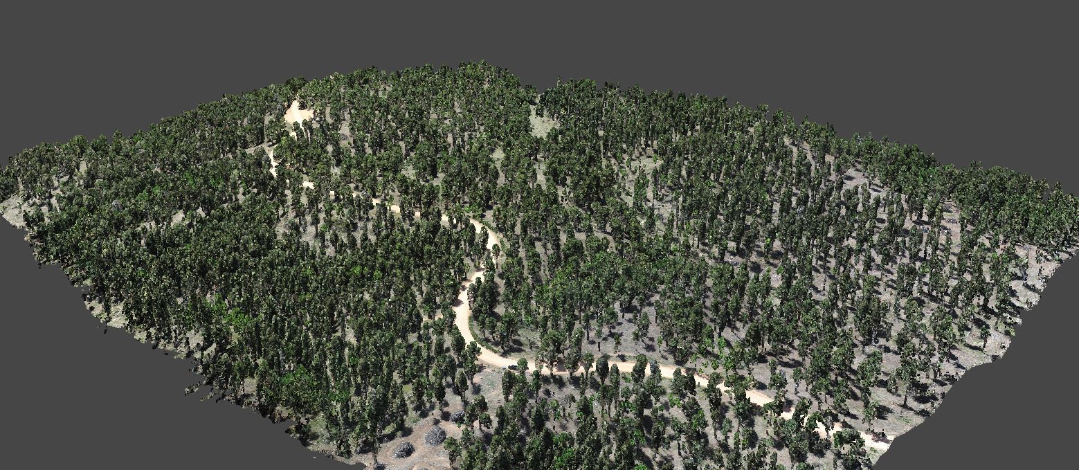
In order to know what we can use GEDI data for, we need to get an idea of how well it estimates 3D forest structure, like maximum canopy height, percent cover, and more. We can leverage aerial LiDAR (ALS) or Structure from Motion (SfM) derived point cloud data to validate GEDI waveform data. Here is an example of some high density ALS from the Kaibab National Forest in Arizona collected in 2019.

The idea behind validating GEDI footprint data with ALS data is to use ALS data as “truth”, and directly compare ALS forest structure metrics to GEDI forest structure metrics. We just need to make sure that we use ALS data collected around the same time as the GEDI footprint data.
- Step 1: Download and process GEDI footprints that overlap with the extent of your desired LiDAR files
- Step 2: Clip GEDI footprint extents out of the LiDAR files, classify ground, and height normalize to remove terrain
- Step 3: Calculate forest structure metrics for each GEDI-ALS footprint extent
- Step 4: Visualize GEDI metrics for a given footprint to get a better idea of what GEDI data is
Validation methods
Step 1:
We downloaded and processed 2020 GEDI footprint data for all of Colorado. Next, we checked the footprint overlap with Unmanned Aerial System (UAS) based SfM point cloud dataset collected in summer of 2021.
- Here is the extent of the UAS derived Structure from Motion Point Cloud (420473.2 m², 310+ million points)
Step 2:
Next, we clipped the SfM point cloud data to the extent of the GEDI footprints, resulting in only four footprints. We then classified ground using a cloth simulation filter from the lidR package in R, and height normalized using a k nearest neighbor approach with inverse distance weighting.
Here are the clipped, ground classified, height normalized footprints from above

Here are the same footprints from the side

Step 3:
Next, we calculated maximum tree height and percent canopy cover for each SfM point cloud footprint through a series of steps:
- Step 1: Generate 0.25m canopy height model (CHM) rasters for each SfM footprint
- Step 2: Use local maximum filter with a variable window radius to detect all tree locations and heights above 2m
- Step 3: Automatically delinate delineate tree crowns with marker controlled watershed algorithm for each detected tree
- Step 4: Summarize single tree locations and heights to determine maximum tree height within footprint extent
- Step 5: Aggregate all crown polygons into a single polygon, and calculate the area of the aggreated polygon
- Step 6: Divided the area of the tree only polygon by the total area of the footprint to estimate percent canopy cover
Below you can see a sfM footprint on the left, the rasterized CHM in the middle, and the tree locations (black crosses) and crown polygons (black outlines) overlaid on the CHM on the right

Step 4:
Lets explore a way to visualize a 2D comparison of SfM single tree detected canopy cover vs GEDI percent canopy cover.
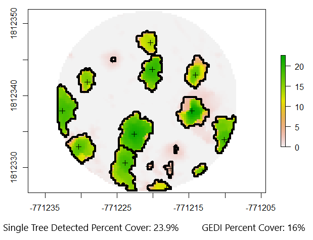
The single tree detected cover looks about right when summarizing the canopy areas visually, and the GEDI percent cover is also similar. We need to keep in mind that GEDI footprint locations can vary by up to 10m compared to their reported locations in the version 2 data release, so its possible that this GEDI footprint was just off a little bit and thats why we see a lower percent canopy cover.
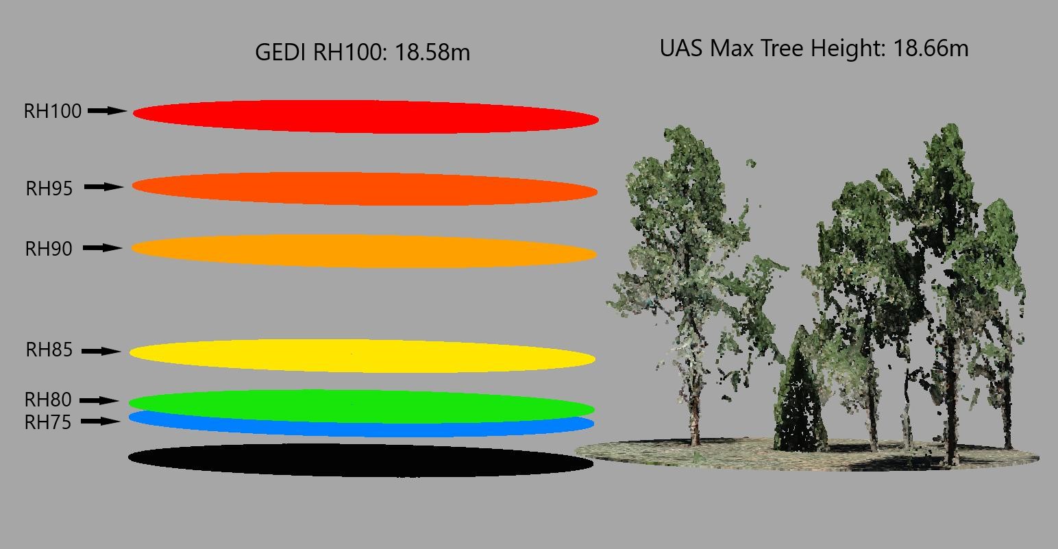
Lets visualize max canopy height for point cloud data and GEDI footprint data.
Below, we have a clipped SfM point cloud for a given GEDI footprint on the right, and on the left, we have 6 disks representing GEDI relative height metrics. The top disk (red) depicts RH100. As you can see, the max tree height is very similar to the GEDI RH100 metric.
 Recomended Citation: Swayze, Neal; Vogeler, Jody (2021): Visualization of GEDI relative height metrics in 3D space. figshare. Media. https://doi.org/10.6084/m9.figshare.16985575.v1
Visualizing in 3D Space
Below are two video examples of the clipped UAS/GEDI RH metrics footprints in three dimensional space. We can apply this same processing method across thousands of footprints as well. As you can see, the GEDI RH100 matches the tops of trees fairly well across many footprints.
Recomended Citation: Swayze, Neal; Vogeler, Jody (2021): Visualization of GEDI relative height metrics in 3D space. figshare. Media. https://doi.org/10.6084/m9.figshare.16985575.v1
Recomended Citation: Swayze, Neal; Vogeler, Jody (2021): Visualization of GEDI relative height metrics in 3D space. figshare. Media. https://doi.org/10.6084/m9.figshare.16985575.v1
The NASA Global Ecosystem Dynamics Investigation (aka GEDI) is a recent NASA project using high resolution laser ranging observations to model the three dimensional structure of the earth. The GEDI instrument makes precise measurements of forest canopy height, canopy vertical structure, and surface elevation.
The GEDI sensor sends out pulses of laser light, which travel from the sensor to the earths surface, interact with the ground/vegetation, then a certain proportion of the light pulse returns and is captured by the sensors telescope. The time between the emission and reception of the light pulse is then used to calculate a waveform (distribution). These waveforms are further processed to estimate an elevation, ground surface, and a variety of canopy metrics, including relative height, percent cover, foliage height diversity, and plant area index.
The goal of the GEDI project will be to investigate data fusions for “scaling-up” GEDI footprint information to landscape scales using additional continuous remote sensing data sources. The landscape scale structure metrics will then be incorporated into habitat modeling for wildlife species of management and conservation interest, and for identifying diversity “hotspots” of these species.
Part of investigating new data comes with the task of visualizing abstract data. Sure, tables and graphs are typical, but what about something a bit more visually appealing?
Downloading and Processing GEDI DATA
-
Step 1: Get a LPDACC Earthdata Login Account (https://urs.earthdata.nasa.gov/users/new)
-
Step 2: Install the rGEDI package in R https://github.com/carlos-alberto-silva/rGEDI and load some other helpful packages
- Lets also create a root directory and some subfolders to organize our data
### Install rGEDI package
install.packages("rGEDI")

### Load Nessesary Packages
library(rGEDI)
library(lidR)
library(data.table)
library(dplyr)
library(sp)
library(sf)

### Set the working directory
rootdir <- ("D:/gedi_example")
dir.create(file.path(rootdir, "gedi_downloads"))
download_dir <- file.path(rootdir, "/gedi_downloads")
dir.create(file.path(rootdir, "gedi_processed"))
processed_data_dir <- file.path(rootdir, "/gedi_processed")
- Step 3: Next we define our desired study area and date range and then use the gedifinder function to find our data
- The gedifinder function returns a string containing the file path to your desired granule file
- You will need to enter your EarthData login credentials when you run the gediDownload line
- The desired GEDI granule file will automatically download to your desired directory
- Pro tip: Go get a cup of coffee, it takes a little while
### Define Study area boundary box coordinates
ul_lat<- -44.0654
lr_lat<- -44.17246
ul_lon<- -13.76913
lr_lon<- -13.67646

### Specifying the date range
daterange=c("2019-07-01","2019-09-23")

### Find the desired granules
gLevel2A <- gedifinder(product="GEDI02_A",ul_lat, ul_lon, lr_lat, lr_lon,version="002",daterange=daterange)
gLevel2A

### Download the desired granule file
gediDownload(filepath=gLevel2A, outdir=download_dir)
- Step 4: Once your file is done downloading, you will need to read it into R
- The below for loop will process through a list of granules to return a .csv and .shp for each granule
### Generating a list of granule files to process from the GEDI downloads folder
setwd(download_dir)
list <- list.files(setwd(download_dir), pattern = "*.h5")
list

### Define the desired beams you want to retain - (these are full power beams)
target_beams <- c("BEAM0101", "BEAM0110", "BEAM1000", "BEAM1011")

### For loop to read in and process the GEDI data
for (i in seq(list)){

  ### Get the first object in the list
  desired_granule <- list[[i]]
  desired_granule

  ### Get an output name
  out_name <- tools::file_path_sans_ext(desired_granule)
  out_name_shp <- paste0(out_name, ".shp")
  out_name_csv <- paste0(out_name, ".csv")

  ### Read in the .h5 file, convert to dataframe object
  setwd(download_dir)
  file = readLevel2A(desired_granule)
  file = getLevel2AM(file)
  file = as.data.frame(file)

  ### Filter the GEDI dataframe to contain desired information
  file = subset(file, select = c(shot_number, beam, degrade_flag, quality_flag,
                                 sensitivity, solar_elevation, lat_lowestmode,
                                 lon_lowestmode, elev_lowestmode, rh0, rh5,
                                 rh10, rh20, rh30, rh40,rh50, rh60, rh65,
                                 rh70, rh75, rh80, rh85, rh90, rh95, rh96,
                                 rh97, rh98, rh99, rh100))

  file = filter(file, ((solar_elevation < 0) &
                         (degrade_flag == 0) &
                         (quality_flag == 1) &
                         (beam %in% target_beams) &
                         (sensitivity >= 0.95) ) )

  ### Convert the gedi dataframe to a spatial points object, reproject to EPSG 5070
  file_spdf = SpatialPointsDataFrame(cbind(file$lon_lowestmode,file$lat_lowestmode), data=file)
  proj4string(file_spdf) = CRS("+init=epsg:4326")
  file_spdf <- spTransform(file_spdf, CRS("+init=epsg:5070"))
  proj4string(file_spdf) = CRS("+init=epsg:5070")

  ### Write out a shapefile object
  out_shp <- st_as_sf(file_spdf)
  setwd(processed_data_dir)
  st_write(out_shp, out_name_shp, append=FALSE)

  ### Convert back to dataframe, write out .csv file
  file <- as.data.frame(file_spdf)
  setwd(processed_data_dir)
  fwrite(file, file = out_name_csv, sep = ",")

  ### Clean up your working environment to save memory
  rm(file, out_name, desired_granule)
  gc()
}
- You have sucsessfully processed your first GEDI granule into a more usable format!
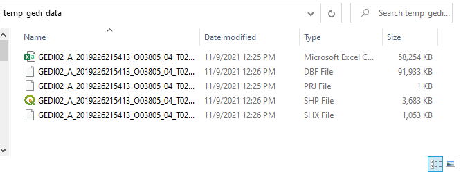
- Your processing folder should look similar to the image below
#
Visualizing GEDI Data
- Step 5: Lets use QGIS to visualize the shapefile:
#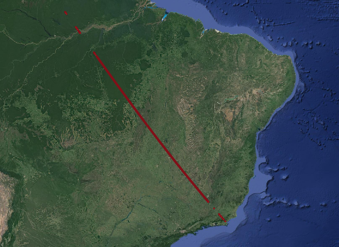
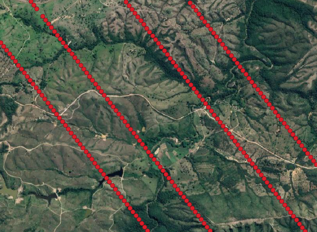
- This is the filtered GEDI footprint data. Zooming in shows us a nice distrubtion of gedi footprints for the four beams.
- Step 6: We now have a .csv of filtered GEDI data ready to work with. Lets convert the .csv file to a .las file using the rlas package
### Read in the processed CSV file
setwd(processed_data_dir)
gedi_data <- fread("GEDI02_A_2019226215413_O03805_04_T02285_02_003_01_V002.csv")
gedi_data <- as.data.frame(gedi_data)
gedi_data

### Creating a las file for the extracted X, Y, and Z, writing out file
x = round(gedi_data$coords.x1, digits = 3)
y = round(gedi_data$coords.x2, digits = 3)
z = round(gedi_data$elev_lowestmode, digits = 3)

### Write out the las file using the rlas package
lasdata = data.frame(X = x, Y = y, Z = z)
lasheader = header_create(lasdata)
file = file.path(processed_data_dir, "gedi_true_elevation.las")
setwd(processed_data_dir)
write.las(file, lasheader, lasdata)
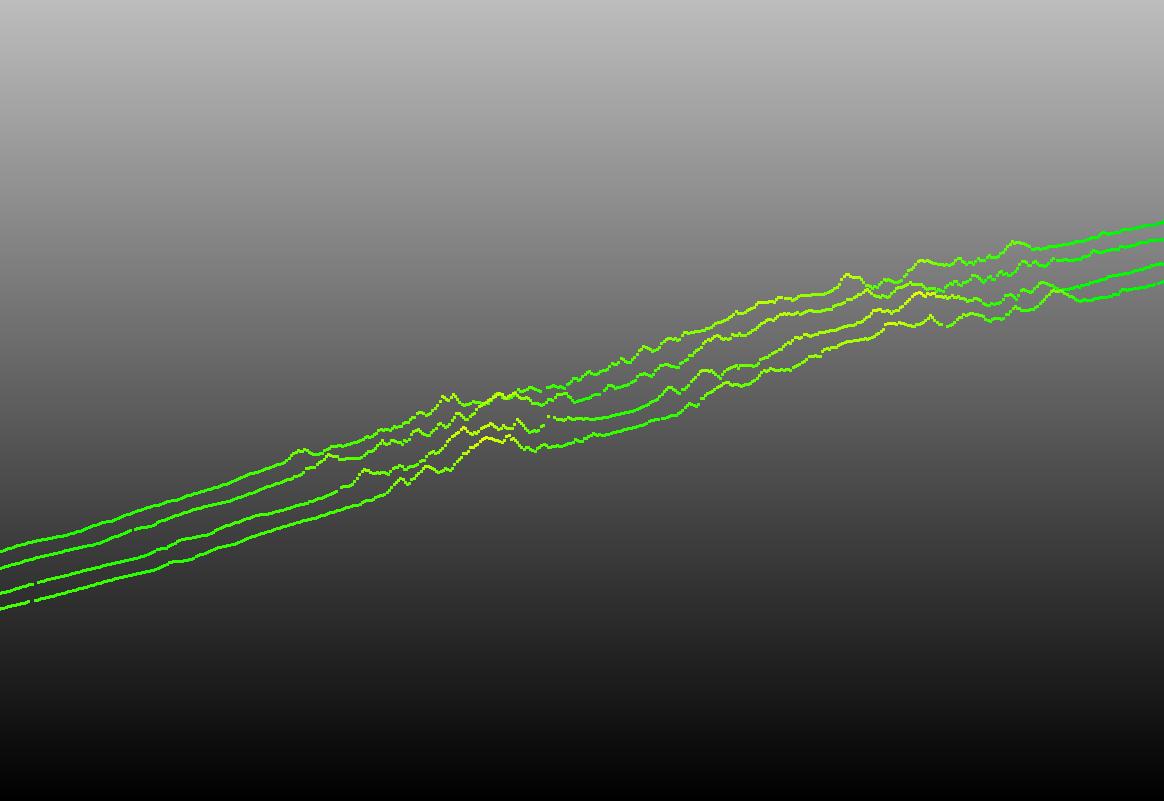
- Step 7. Now you have a .las file containing all of your GEDI footprints, which you can visualize in CloudCompare
- Now we can see the elevation of the GEDI footprints in 3D space for each beam track!
#
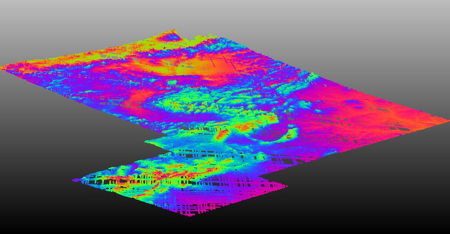
- This method can be adapted to visualize GEDI data in all sorts of new ways. Here is a 3D example of GEDI footprint elevations across our GEDI project study area (spanning Colorado, Wyoming, Idaho, Oregon, Washington, and Montana) Each point in this image is a GEDI waveform footprint, scaled on the Z axis as elevation.
#
- Hopefully this post helps someone get more comfortable with basic processing and visualization of GEDI data!