GEDI Data Processing and Visualization - Post 2

December 20, 2021

In our previous post, we demonstrated a basic outline for processing and visualizing GEDI data.

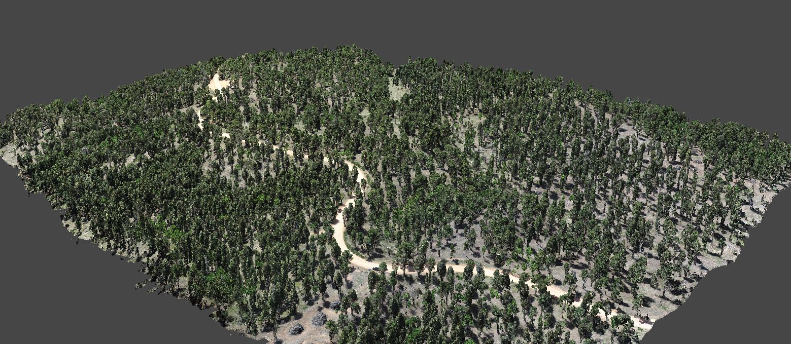
In order to know what we can use GEDI data for, we need to get an idea of how well it estimates 3D forest structure, like maximum canopy height, percent cover, and more. We can leverage aerial LiDAR (ALS) or Structure from Motion (SfM) derived point cloud data to validate GEDI waveform data. Here is an example of some high density ALS from the Kaibab National Forest in Arizona collected in 2019.

title

The idea behind validating GEDI footprint data with ALS data is to use ALS data as “truth”, and directly compare ALS forest structure metrics to GEDI forest structure metrics. We just need to make sure that we use ALS data collected around the same time as the GEDI footprint data.

Basic workflow for comparing ALS to GEDI footprint observations

Step 1: Download and process GEDI footprints that overlap with the extent of your desired LiDAR files
Step 2: Clip GEDI footprint extents out of the LiDAR files, classify ground, and height normalize to remove terrain
Step 3: Calculate forest structure metrics for each GEDI-ALS footprint extent
Step 4: Visualize GEDI metrics for a given footprint to get a better idea of what GEDI data is

Validation methods

Step 1:

We downloaded and processed 2020 GEDI footprint data for all of Colorado. Next, we checked the footprint overlap with Unmanned Aerial System (UAS) based SfM point cloud dataset collected in summer of 2021.

Here is the extent of the UAS derived Structure from Motion Point Cloud (420473.2 m², 310+ million points)

Step 2:

Next, we clipped the SfM point cloud data to the extent of the GEDI footprints, resulting in only four footprints. We then classified ground using a cloth simulation filter from the lidR package in R, and height normalized using a k nearest neighbor approach with inverse distance weighting.

Here are the clipped, ground classified, height normalized footprints from above

title

Here are the same footprints from the side

title

Step 3:

Next, we calculated maximum tree height and percent canopy cover for each SfM point cloud footprint through a series of steps:

Step 1: Generate 0.25m canopy height model (CHM) rasters for each SfM footprint
Step 2: Use local maximum filter with a variable window radius to detect all tree locations and heights above 2m
Step 3: Automatically delinate delineate tree crowns with marker controlled watershed algorithm for each detected tree
Step 4: Summarize single tree locations and heights to determine maximum tree height within footprint extent
Step 5: Aggregate all crown polygons into a single polygon, and calculate the area of the aggreated polygon
Step 6: Divided the area of the tree only polygon by the total area of the footprint to estimate percent canopy cover

Below you can see a sfM footprint on the left, the rasterized CHM in the middle, and the tree locations (black crosses) and crown polygons (black outlines) overlaid on the CHM on the right

title

Step 4:

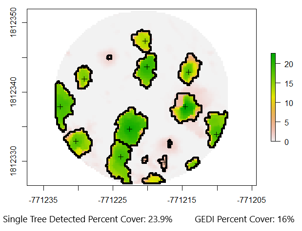
Lets explore a way to visualize a 2D comparison of SfM single tree detected canopy cover vs GEDI percent canopy cover.

title

The single tree detected cover looks about right when summarizing the canopy areas visually, and the GEDI percent cover is also similar. We need to keep in mind that GEDI footprint locations can vary by up to 10m compared to their reported locations in the version 2 data release, so its possible that this GEDI footprint was just off a little bit and thats why we see a lower percent canopy cover.

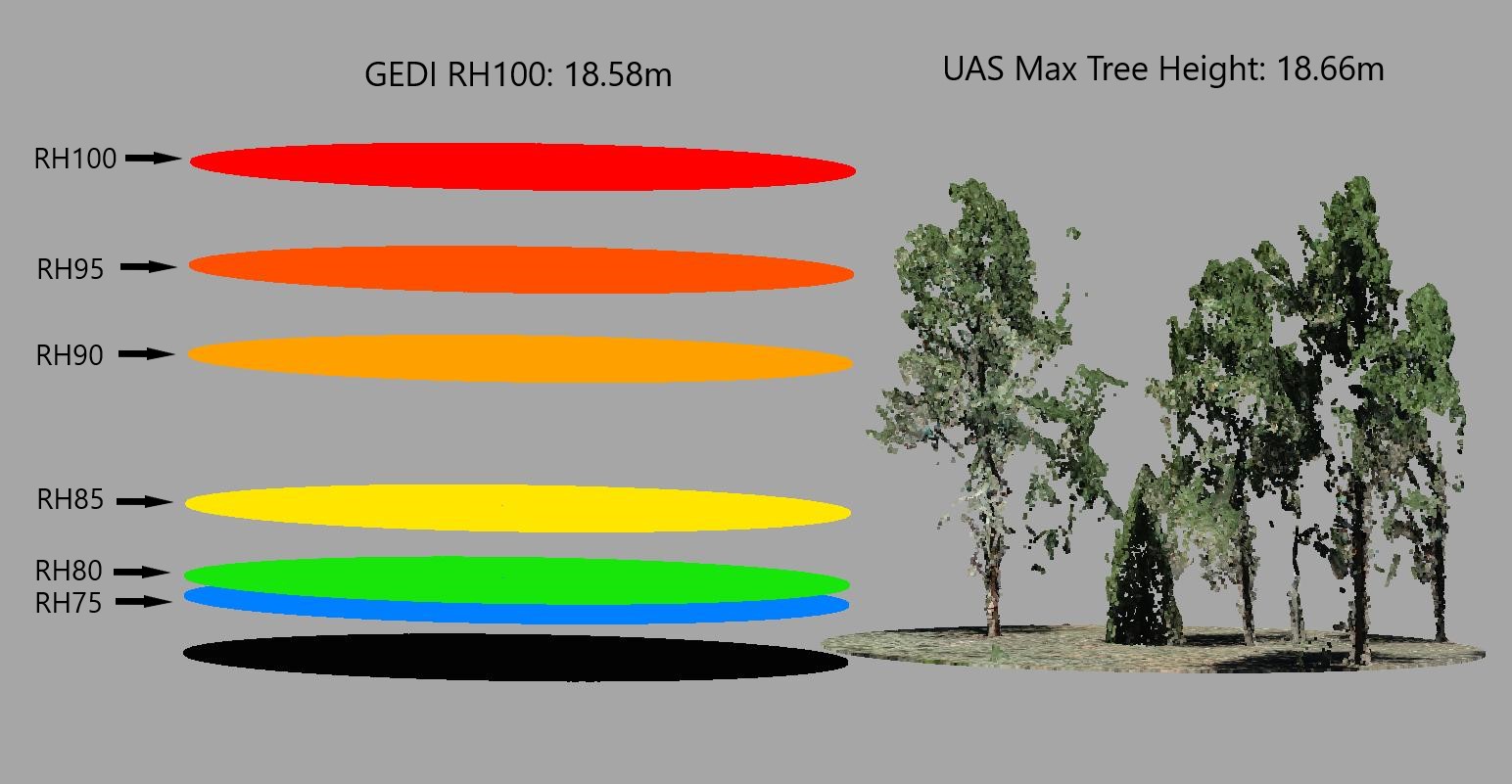
Lets visualize max canopy height for point cloud data and GEDI footprint data.

Below, we have a clipped SfM point cloud for a given GEDI footprint on the right, and on the left, we have 6 disks representing GEDI relative height metrics. The top disk (red) depicts RH100. As you can see, the max tree height is very similar to the GEDI RH100 metric.

title Recomended Citation: Swayze, Neal; Vogeler, Jody (2021): Visualization of GEDI relative height metrics in 3D space. figshare. Media. https://doi.org/10.6084/m9.figshare.16985575.v1

Visualizing in 3D Space

Below are two video examples of the clipped UAS/GEDI RH metrics footprints in three dimensional space. We can apply this same processing method across thousands of footprints as well. As you can see, the GEDI RH100 matches the tops of trees fairly well across many footprints.

Recomended Citation: Swayze, Neal; Vogeler, Jody (2021): Visualization of GEDI relative height metrics in 3D space. figshare. Media. https://doi.org/10.6084/m9.figshare.16985575.v1